Euler Examples

Search

Instable Solutions of Differential Equations

The following demonstrates a common problem of many numerical algorithms. Given exact data, they should deliver a specific solution. But due to rounding errors, the solution forks into a second solution.

As a first example, we consider the differential equation

which looks harmless. Let us solve it for the initial values

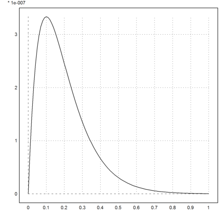
>function f(x,y) := [y[2],100*y[1]]
>x=0:0.01:1; ...
 y=runge("f",x,[1,-10]); ...
 plot2d(x,y[1]):

The exakt solution is

However, the equation has a second solution exp(10*x). The general solution is the following.

>&ode2('diff(y,x,2)=100*y,y,x)

                              10 x        - 10 x
                     y = %k1 E     + %k2 E

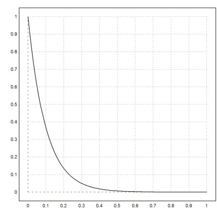
Even the difference to the true solution is very stable, and gets better with larger x.

>plot2d(x,y[1]-exp(-10*x)):

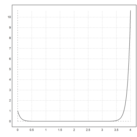
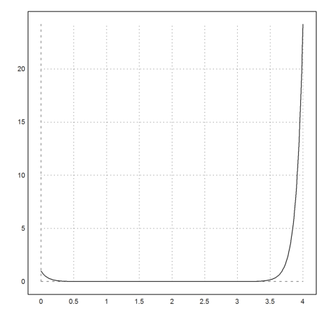
But, if we iterate long enough, the runge algorithm will fork into the second solution (with a negative constant %k2).

>x=0:0.01:4; ...
 y=runge("f",x,[1,-10]); ...
 plot2d(x,y[1]):

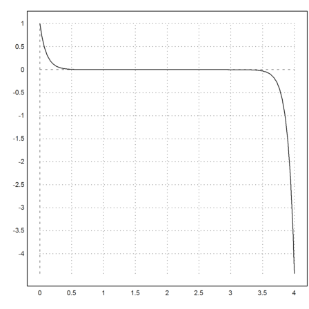
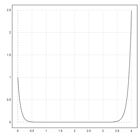
The adaptive Runge method does not help. The behavior is sort of random.

>x=0:0.01:4; ...
 y=adaptiverunge("f",x,[1,-10]); ...
 plot2d(x,y[1]):

Our equation is simply

with the following matrix A.

>A = [0,1;100,0]

            0             1 
          100             0 

The simple Euler method is

>y=sequence("(id(2)+0.01*A).x[:,n-1]",[1;-10],401);
>x=0:0.01:4; plot2d(x,y[1]):

The problem is the Eigenvalue 1.1 of the iteration matrix.

>real(eigenvalues(id(2)+0.01*A))

[1.1,  0.9]

We can try to fix this instability in this simple, linear case in the following way.

We use an implicit equation instead with

In our simple case y'=A*y with a 2x2 matrix A, we get

Thus we solve a linear system in each step.

>B=inv(id(2)-0.01*A/2).(id(2)+0.01*A/2); real(eigenvalues(B))

[1.10526,  0.904762]

>y=sequence("B.x[:,n-1]",[1;-10],401);

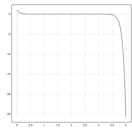
But this algorithm does not help either.

>x=0:0.01:4; plot2d(x,y[1]):

Not even the LSODA algorithm works in this case, since the problem is just the instability of the initial condition. The stiff solvers only make sure that the part which is tending to 0 does indeed tend to 0. In our case, this is not the problem.

>x=0:0.01:4; ...
 y=ode("f",x,[1,-10]); ...
 plot2d(x,y[1]):

Examples